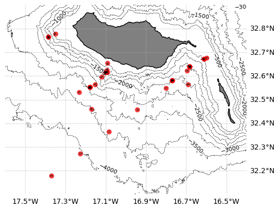
Anton and I have just brought CTD cast number 45 to light. While we are once again shaking freshly tapped bottles with great enthusiasm, I think I can make out question marks in Jamileh’s expression as she smiles good morning to us. That’s what everyone here seems to be thinking: 45 CTD casts already? And many of them in the same place? Why all this? We should know the water once we’ve “measured” it, right? Well, somehow we do.

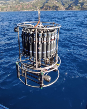
“Our” CTD, which biologists prefer to call a “water sampler”, is moved out of the side of the hangar, lowered and in the basic version measures Conductivity (salinity), Temperature and pressure (Depth) quasi continuously (at 24 Hz), ideally down to the seafloor. In addition, oxygen and fluorescence are measured, which makes it possible to estimate biological productivity (see previous blog entries by Nicole and Manfred). As an addition, water samples can be taken at various depths using the 24 Niskin bottles (Manfred is by far our best customer in this respect). For oceanographers, however, the continuous measurements of temperature and salinity are of crucial importance, as they allow us to see how stable the water is stratified, for example, or to deduce the origin of the water masses and geostrophic currents. This is important information that forms the framework conditions that strongly influence the local ecosystem. In order to achieve maximum precision in the physical measurements, I take water samples myself “only” to calibrate the oxygen and salinity sensors later, but not to analyze the suspicious living beings in it.

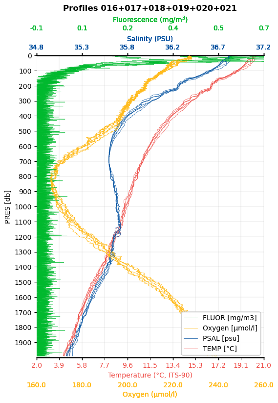
Most of the deployments to date have been close to shore at a depth of about 1500 meters. The following figure shows one of our precious deeper profiles down to a depth of almost 3300 meters. Here, the top 100 meters form the so-called “mixed layer”, in which all measured variables are well mixed by the wind. We observe that the depth of this surface layer varies, but is generally comparatively thick – as is typical for the winter months at these latitudes. At our first station, the mixed layer depth was even around 200m! Temperature (red), salt (blue), oxygen (yellow) and chlorophyll (green) draw practically vertical lines in the diagram. Interestingly, a maximum of chlorophyll often forms exactly at or below the surface layer, which serves as an indicator for the presence of phytoplankton (see Nicole’s and Manfred’s blog entry on “Micro-Creatures”). Although phytoplankton is basically autotrophic, i.e. dependent on sunlight, it can survive in this rather deep layer with very little sunlight. One reason for this is the increased nutrient content in deeper layers.

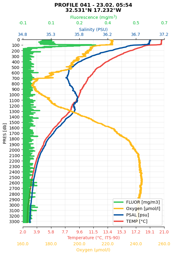
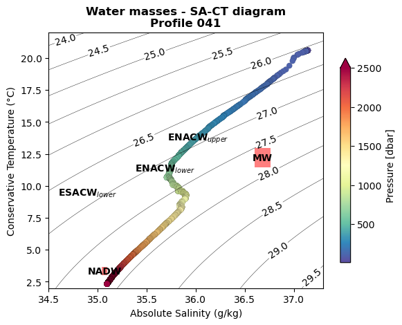
In addition, the pycnocline directly below the mixed layer forms a strong physical barrier to vertical mixing and can practically “trap” organisms that cannot actively swim themselves. The pycnocline is the layer in which the density of the water increases very rapidly with depth (here due to the temperature gradient). These layers contain a wide range of temperature and salt contents and are also called Central Waters. To identify water masses, temperatures and salinities are plotted against each other in a so-called “T-S diagram” (as shown in Figure 4). In our example, you can clearly see that the water around Madeira consists largely of Eastern North Atlantic Central Water (ENACW). This water mass dominates the pycnocline in the large North Atlantic Gyre and is significantly more saline than in the South Atlantic (see Eastern South Atlantic Central Water). In our profile number 41 (Figure 3), however, something else catches the eye. At around 1100m, there is a nose with a significantly higher salinity, which does not seem to match the linear Central Water. The influence of the Mediterranean Water (MW) is noticeable here, which has a particularly high salt content due to the predominantly high evaporation and low precipitation in the Mediterranean region.

Due to this high salt content, it manifests itself at greater depths, typically around 1100m to 1200m, despite the warm temperatures. However, we can also see in the T-S diagram that the Mediterranean water in the south of Madeira is already somewhat more mixed, i.e. less warm and saline than directly at the outflow of the Mediterranean. Even further down, which we can observe particularly well at our deeper CTD stations around 3000m, resides the famous North Atlantic Deep Water (NADW). This is formed by, for instance, deep convection in the North Atlantic and plays a central role in global thermohaline circulation and climate dynamics. Although constituting deep water, it is comparatively “young” and therefore rich in oxygen (we like to say “well ventilated”) and forms a contrast to the oxygen minimum, which we observe here around Madeira at around 800-900 meters. This minimum zone is formed by respiration of the sunken organic material, e.g. from the sunlight-dependent phytoplankton in the uppermost ~150 meters. Compared to the large known oxygen minimum zones in the subtropical eastern Atlantic and Pacific, however, there is still comparatively abundant oxygen.

Now, we know the profile of a single CTD station a little better. Basically, this one is actually fairly representative of the other 44, so the question of why Anton and I keep “driving CTDs” like madmen remains unanswered. However, if we take a closer look, we can see that the temperature and salinity profiles are not completely “smooth”. In fact, we discover small wavelike deviations. Measurement inaccuracies? No. It is internal waves that bring “life” to the profiles. Internal waves can occur in any stratified medium, i.e. fluids in which the density is not constant. There are two restoring forces that act on internal waves in the ocean: Gravity and the Coriolis force. The main drivers of internal waves are the tides (such as ebb and flow), closely followed by wind. We know that internal waves play a crucial role in energy transport in the ocean. Like ordinary surface waves, internal waves can also break. When they do, mixing takes place. This in turn can transport nutrients and thereby influence biological productivity. The interaction of internal waves with topography (i.e. islands such as Madeira) and currents is very complex and not yet fully understood. By using a large number of stations at different times (and tidal stages), we obtain a better spatial and temporal resolution of the internal wave field and improve our understanding. That’s also why we are fans of so-called “yo-yo CTDs”. Just like a real yo-yo, we move the CTD up and down several times in direct succession at one and the same location.

In the figure above, we have plotted six directly consecutive profiles of a “CTD yo-yo” on top of each other. You can see that the profiles deviate more from each other at some depths and not at others (nodal points). The most impressive influence is exerted by internal waves on the mixed layer depth, which can vary by several tens of meters within minutes.

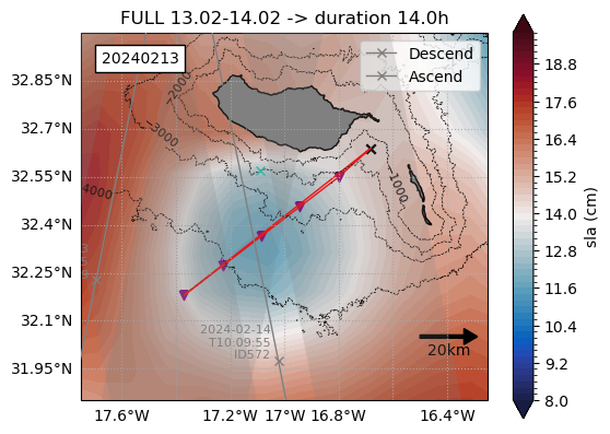
There is a particular thrill when the “Eddy hunt” is called for. That sounds more martial than it is meant to be. Eddies are oceanic vortices that reach a diameter of about 50 km around Madeira, interact with topography (islands) and internal waves and are known to have an impact on biodiversity. They develop over a period of days/weeks and are unfortunately hardly predictable. Therefore, we check satellite and model data for the region daily to identify a possible feature and, if possible, sample in situ with Merian. Strong eddies can generate a signal in sea level, surface temperatures and chlorophyll, recognizable via satellites. Our colleagues from the Oceanographic Institute of Madeira are helping us on site by providing the regional satellite and model data (see https://oomdata.arditi.pt/msm126/). Overall, it is impressive how well the collaboration on board and beyond works! One “eddy hunt” has already taken place on the night of February 13-14. However, the satellite signal was weak, and accordingly we were unable to detect a strong, coherent eddy In Situ with our shipboard ADCP (Acoustic Doppler Current Profiler, which measures ocean currents down to a depth of almost 1000m). (Side note: However, another exciting feature (presumably a strong internal wave) was identified in the surface layer, which we are now analyzing.)

In one of the following contributions, we want to prove to you that our beloved CTD is something very special in purely “objective” terms thanks to sophisticated tuning, including high-resolution camera systems. Then we’ll explain why Anton, although he’s not a physical oceanographer, also likes to drive “CTD yo-yos” and there will finally be photos of aquatic animals again!

Greetings from on board RV MARIA S. MERIAN,

Marco Schulz und Anton Theileis